Cross-Validation

Universidad Central

Maestría en analítica de datos

Métodos estadísticos para analítica de datos.

Docente: Luis Andrés Campos Maldonado.

import warnings
warnings.filterwarnings("ignore")

import numpy as np
import pandas as pd
import matplotlib.pyplot as plt
from pprint import pprint
from sklearn.compose import ColumnTransformer
from sklearn.preprocessing import OneHotEncoder, label_binarize
from sklearn.pipeline import Pipeline
from sklearn.linear_model import LogisticRegression
from sklearn.ensemble import RandomForestClassifier
from sklearn.metrics import roc_auc_score, roc_curve, auc
from sklearn.model_selection import (
    GridSearchCV,
    RandomizedSearchCV,
    train_test_split,
    cross_validate
)

plt.style.use("ggplot")
plt.rcParams["figure.figsize"] = (15,6)
url_base = "https://raw.githubusercontent.com/lacamposm/Metodos-Estadisticos/main/data/"

Cross-Validation.

Pensemos en la siguiente situación de la vida “real”:

Usted está estudiando para un examen y ha logrado memorizar muchos de los ejercicios que ha desarrollado como preparación, dado que usted “memorizó” (no-generalizó) seguramente en un exámen con las mismas preguntas (que usted ya “memorizó”) tendrá un buen resultado. Siguiendo en la analogía, ¿cómo cree que será su calificación si el exámen tiene un grupo de preguntas que usted nunca ha estudiado? Recuerde que solo “memorizó”…

Suponga ahora que está construyendo un modelo de machine learning, ¿cómo puede eliminar el problema de “memorizar” del sistema? Intuitivamente, parece completamente lógico dejar un conjunto de datos reservados (set_test) que NO hará parte del entrenamiento del modelo y luego de entrenado dicho modelo aplicarlo sobre los datos reservados para ver que tan bien se comporta. En este caso, usaría la mayoría de los datos para ajustar el modelo (entrenar) y usar una porción más pequeña para probar el modelo. ¿Qué tan diferente sería la evaluación si selecciona una muestra reservada diferente?

La técnica de cross validation amplía la idea de una muestra reservada a múltiples muestras reservas secuenciales.

1. Reserve \(1/k\) de los datos como muestra reservada.

2. Entrene el modelo con los datos restantes.

3. Aplique (score) el modelo a la reserva de \(1/k\) y registre la métrica(s) de evaluación del modelo que desea.

4. Restaure el primer \(1/k\) de los datos y reserve el siguiente \(1/k\) (excluyendo cualquier registro que fue elegido la primera vez).

5. Repita los pasos 2 y 3.

6. Repita hasta que se haya utilizado cada registro en la parte reservada.

7. Promediar o combinar las métricas de evaluación del modelo.

La división de los datos en la muestra de entrenamiento y la muestra reservada también se denomina un fold.

Para hacer uso de esta técnica podemos usar las siguientes herramientas:

1. sklearn.model_selection.StratifiedKFold

2. sklearn.model_selection.KFold

3. sklearn.model_selection.cross_validate

# Preparamos la Data
df_to_model = pd.read_parquet(url_base + "Logistic_Regression_1.parquet",)
df_to_model.drop_duplicates(inplace=True)
df_to_model["tasa_de_interes"] = df_to_model["tasa_de_interes"].str.replace("%", "").astype("float")
df_to_model.drop(columns=["estado_de_verificacion"], inplace=True)
df_to_model

	estado_del_prestamo	ingreso_anual	anios_de_experiencia_laboral	tenencia_de_vivienda	tasa_de_interes	monto_del_prestamo	proposito	plazo	calificacion
0	completamente_pagado	24000.0	10+ años	alquiler	10.65	5000	tarjeta_de_credito	36 meses	B
1	dado_de_baja	30000.0	< 1 año	alquiler	15.27	2500	auto	60 meses	C
2	completamente_pagado	12252.0	10+ años	alquiler	15.96	2400	pequeno_negocio	36 meses	C
3	completamente_pagado	49200.0	10+ años	alquiler	13.49	10000	otro	36 meses	C
4	completamente_pagado	80000.0	1 año	alquiler	12.69	3000	otro	60 meses	B
...	...	...	...	...	...	...	...	...	...
38700	completamente_pagado	110000.0	4 años	hipoteca	8.07	2500	remodelacion_del_hogar	36 meses	A
38701	completamente_pagado	18000.0	3 años	alquiler	10.28	8500	tarjeta_de_credito	36 meses	C
38702	completamente_pagado	100000.0	< 1 año	hipoteca	8.07	5000	consolidacion_de_deudas	36 meses	A
38703	completamente_pagado	200000.0	< 1 año	hipoteca	7.43	5000	otro	36 meses	A
38704	completamente_pagado	22000.0	< 1 año	propia	13.75	7500	consolidacion_de_deudas	36 meses	E

38689 rows × 9 columns

categorical_features = [col for col in df_to_model.select_dtypes(exclude=np.number).columns if col != "estado_del_prestamo"]
numeric_features = [col for col in df_to_model.columns if col not in categorical_features and col != "estado_del_prestamo"]

preprocessor = ColumnTransformer(
    transformers=[
        ("onehot", OneHotEncoder(drop="first"), categorical_features),
        ("num", "passthrough", numeric_features)        
    ]
)

X = df_to_model[categorical_features + numeric_features]
X = preprocessor.fit_transform(X)
y = label_binarize(df_to_model["estado_del_prestamo"], classes=["dado_de_baja", "completamente_pagado"])
X_train, X_test, y_train, y_test = train_test_split(X, y, test_size=0.2, stratify=y, random_state=123)

Modelo Logistic Regression.

# Logistic Regression con sklearn.
model_lr = LogisticRegression(C=1e10, solver="newton-cg", fit_intercept=True, random_state=123)
model_lr.fit(X_train,y_train)

predict_proba_train = model_lr.predict_proba(X_train)[:,1]
predict_proba_test = model_lr.predict_proba(X_test)[:,1]

print(f"Logistic Regression AUC Train = {roc_auc_score(y_train, predict_proba_train):.3f}")
print(f"Logistic Regression AUC Test = {roc_auc_score(y_test, predict_proba_test):.3f}")

Logistic Regression AUC Train = 0.692
Logistic Regression AUC Test = 0.688

cv_results_lr = cross_validate(
    model_lr,
    X_train,
    y_train,
    cv=5,
    scoring=("roc_auc","f1"),
    return_train_score=True,
)

pd.DataFrame(cv_results_lr)

	fit_time	score_time	test_roc_auc	train_roc_auc	test_f1	train_f1
0	2.472225	0.010654	0.695260	0.690147	0.924080	0.924381
1	2.239501	0.010728	0.669770	0.696917	0.923786	0.924422
2	2.684600	0.005953	0.705949	0.687860	0.924389	0.924411
3	1.066561	0.005805	0.685432	0.692836	0.924441	0.924251
4	1.169047	0.004714	0.680731	0.694208	0.924509	0.924325

train_lr, test_lr = cv_results_lr["train_roc_auc"], cv_results_lr["test_roc_auc"]
means_lr = (train_lr.mean(), test_lr.mean())
# Para los límites en el eje y
values_aucs_lr = np.concatenate((train_lr, test_lr), axis=None)
min_y, max_y = values_aucs_lr.min() -0.01 , values_aucs_lr.max()+ 0.01
##
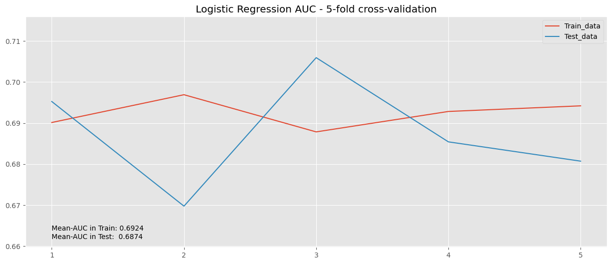
plt.plot(cv_results_lr["train_roc_auc"], label="Train_data")
plt.plot(cv_results_lr["test_roc_auc"], label = "Test_data")
plt.title("Logistic Regression AUC - 5-fold cross-validation")
plt.legend()
plt.text(0, min_y + 4e-03, f"Mean-AUC in Train: {means_lr[0]:.4f}")
plt.text(0, min_y + 2e-03, f"Mean-AUC in Test:  {means_lr[1]:.4f}")
plt.ylim(min_y, max_y)
plt.xticks(np.arange(0,5), np.arange(1,6))
plt.show()

Modelo Random Forrest.

preprocessor = ColumnTransformer(
    transformers=[
        ("onehot", OneHotEncoder(), categorical_features),
        ("num", "passthrough", numeric_features)        
    ]
)

X = df_to_model[categorical_features + numeric_features]
X = preprocessor.fit_transform(X)
y = label_binarize(df_to_model["estado_del_prestamo"], classes=["dado_de_baja", "completamente_pagado"])
X_train, X_test, y_train, y_test = train_test_split(X, y, test_size=0.2, stratify=y, random_state=123)

model_rf = RandomForestClassifier(n_estimators=100, max_depth=3, random_state=123)
model_rf.fit(X_train,y_train)

predict_proba_train = model_rf.predict_proba(X_train)[:,1]
predict_proba_test = model_rf.predict_proba(X_test)[:,1]

print(f"Random Forrest AUC Train = {roc_auc_score(y_train, predict_proba_train):.3f}")
print(f"Random Forrest AUC Test = {roc_auc_score(y_test, predict_proba_test):.3f}")

Random Forrest AUC Train = 0.683
Random Forrest AUC Test = 0.685

# cross_validate en RandomForrest.
cv_results_rf = cross_validate(
    model_rf,
    X_train,
    y_train,
    cv=5,
    scoring=("roc_auc","f1"),
    return_train_score=True,
    verbose=3
)

[CV] END  f1: (train=0.924, test=0.924) roc_auc: (train=0.685, test=0.677) total time=   1.2s
[CV] END  f1: (train=0.924, test=0.924) roc_auc: (train=0.689, test=0.661) total time=   1.1s
[CV] END  f1: (train=0.924, test=0.924) roc_auc: (train=0.682, test=0.694) total time=   0.9s
[CV] END  f1: (train=0.924, test=0.924) roc_auc: (train=0.684, test=0.681) total time=   0.7s
[CV] END  f1: (train=0.924, test=0.924) roc_auc: (train=0.685, test=0.681) total time=   0.7s

train_lr, test_lr = cv_results_rf["train_roc_auc"], cv_results_rf["test_roc_auc"]

values_aucs_lr = np.concatenate((train_lr, test_lr), axis=None)
min_y, max_y = values_aucs_lr.min() -0.01 , values_aucs_lr.max()+ 0.01
means_rf = (train_lr.mean(), test_lr.mean())

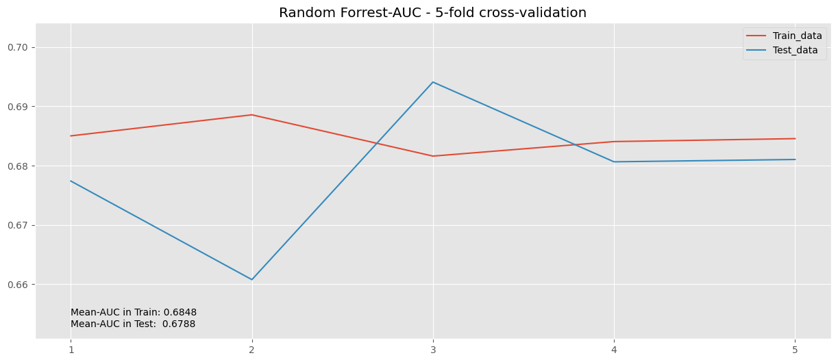
plt.plot(cv_results_rf["train_roc_auc"], label = "Train_data")
plt.plot(cv_results_rf["test_roc_auc"], label = "Test_data")
plt.title("Random Forrest-AUC - 5-fold cross-validation")
plt.legend()
plt.text(0, min_y + 4e-03, f"Mean-AUC in Train: {means_rf[0]:.4f}")
plt.text(0, min_y + 2e-03, f"Mean-AUC in Test:  {means_rf[1]:.4f}")
plt.ylim(min_y, max_y)
plt.xticks(np.arange(0,5),np.arange(1,6))
plt.show()

Búsqueda de parámetros.

Vamos a hacer uso de: sklearn.model_selection.GridSearchCV

# 1 minuto 30 segundos aprox. corriendo.
rf_model = RandomForestClassifier()
params = {
    "n_estimators": [50, 75, 100, 150, 200], 
    "max_depth": [3, 4, 5], 
    "criterion": ["gini", "entropy"],
    "min_samples_split" : [150, 200, 300]
}

clf_rf = GridSearchCV(
    rf_model, 
    params, 
    scoring="roc_auc", 
    cv=3, 
    n_jobs=-1,
    return_train_score=True
)

best_model_grid = clf_rf.fit(X_train,  y_train.ravel())
print("Mejores parametros:\n")
print(best_model_grid.best_params_)

print(f'Random Forrest AUC (Train)= {roc_auc_score(y_train, best_model_grid.predict_proba(X_train)[:,1]):.4f}')
print(f'Random Forrest AUC (Test)= {roc_auc_score(y_test, best_model_grid.predict_proba(X_test)[:,1]):.4f}')

Mejores parametros:

{'criterion': 'gini', 'max_depth': 5, 'min_samples_split': 150, 'n_estimators': 75}
Random Forrest AUC (Train)= 0.6939
Random Forrest AUC (Test)= 0.6899

print("Merojes parametros GridSearchCV:\n")
pprint(clf_rf.best_params_)
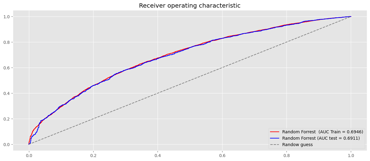
clf_best = clf_rf.best_estimator_.fit(X_train,y_train)

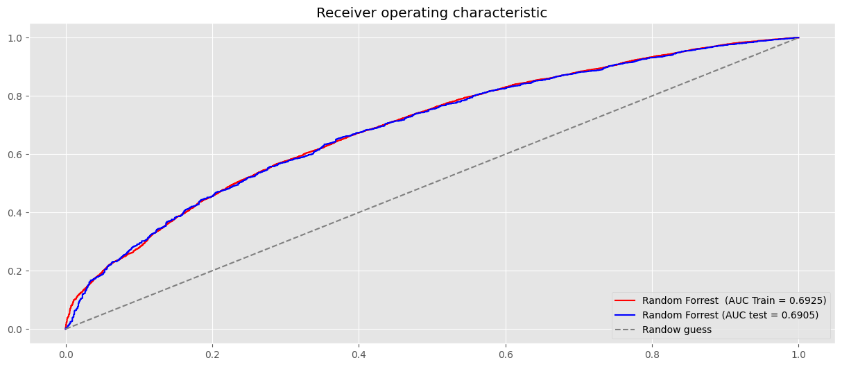
# Curva de ROC en el set de Train.
probas_train = clf_best.predict_proba(X_train)[:,1]
fpr, tpr, _ = roc_curve(y_train, probas_train)
plt.plot(fpr, tpr, label=f"Random Forrest  (AUC Train = {auc(fpr, tpr):.4f})", color="r")

# Curva de ROC en el set de test.
probas_test = clf_best.predict_proba(X_test)[:,1]
fpr_test, tpr_test, _ = roc_curve(y_test, probas_test)
plt.plot(fpr_test, tpr_test, label=f"Random Forrest (AUC test = {auc(fpr_test, tpr_test):.4f})", color="b")

plt.plot((0,1), (0,1), ls = "--", color = "grey", label = "Randow guess")
plt.legend(loc="lower right")
plt.title("Receiver operating characteristic")
plt.show()

Merojes parametros GridSearchCV:

{'criterion': 'gini',
 'max_depth': 5,
 'min_samples_split': 150,
 'n_estimators': 75}

Vamos a hacer uso de: sklearn.model_selection.RandomizedSearchCV

rf_model = RandomForestClassifier()

params = {
    "max_depth": [n for n in range(2, 15)], 
    "criterion": ["gini", "entropy", "log_loss"], 
    "min_samples_split" : [100 + 10*n for n in range(0, 28, 5)],
    "n_estimators":[100 + n for n in range(5, 101, 2)]
}

clf_rf2 = RandomizedSearchCV(
    rf_model,
    params,
    random_state=0,
    scoring="roc_auc",
    cv=5,
    n_iter=10,
    n_jobs=-1,
    return_train_score=True
)

best_model_random = clf_rf2.fit(X_train, y_train.ravel())
print(best_model_random.best_params_)

print(f'Random Forrest AUC (Train)= {roc_auc_score(y_train, best_model_random.predict_proba(X_train)[:,1]):.4f}')
print(f'Random Forrest AUC (Test)= {roc_auc_score(y_test, best_model_random.predict_proba(X_test)[:,1]):.4f}')

{'n_estimators': 153, 'min_samples_split': 200, 'max_depth': 12, 'criterion': 'entropy'}
Random Forrest AUC (Train)= 0.7343
Random Forrest AUC (Test)= 0.6934

X = df_to_model[categorical_features + numeric_features]
y = label_binarize(df_to_model["estado_del_prestamo"], classes=["dado_de_baja", "completamente_pagado"])
X_train, X_test, y_train, y_test = train_test_split(X, y, test_size=0.2, stratify=y, random_state=123)

preprocessor = ColumnTransformer(
    transformers=[
        ("onehot", OneHotEncoder(), categorical_features),
        ("num", "passthrough", numeric_features)        
    ]
)

clf_pipeline_full = Pipeline(steps=[
    ("preprocessor", preprocessor),
    ("classifier", RandomForestClassifier())
])

params = {    
    "classifier__max_depth": [2, 3, 4, 5, 6],
    "classifier__criterion": ["gini", "entropy", "log_loss"],
    "classifier__min_samples_split": [300 + 50 * n for n in range(0, 28)],
    "classifier__n_estimators": [50 + n for n in range(10, 201, 10)],
    "classifier__max_features": ["sqrt", "log2"],
    "classifier__min_samples_leaf": [2, 3, 4, 6, 8]
}

clf = RandomizedSearchCV(
    clf_pipeline_full,
    params,
    n_iter=20,
    scoring="roc_auc",
    cv=3,
    n_jobs=-1,
    random_state=0,
    return_train_score=True
)

search = clf.fit(X_train, y_train.ravel())

print("Merojes parametros RandomizedSearchCV:\n")
pprint(search.best_params_)
clf_best = search.best_estimator_.fit(X_train,y_train)

# Curva de ROC en el set de Train.
probas_train = clf_best.predict_proba(X_train)[:,1]
fpr, tpr, _ = roc_curve(y_train, probas_train)
plt.plot(fpr, tpr, label=f"Random Forrest  (AUC Train = {auc(fpr, tpr):.4f})", color="r")

# Curva de ROC en el set de test.
probas_test = clf_best.predict_proba(X_test)[:,1]
fpr_test, tpr_test, _ = roc_curve(y_test, probas_test)
plt.plot(fpr_test, tpr_test, label=f"Random Forrest (AUC test = {auc(fpr_test, tpr_test):.4f})", color="b")

plt.plot((0,1), (0,1), ls = "--", color = "grey", label = "Randow guess")
plt.legend(loc="lower right")
plt.title("Receiver operating characteristic")
plt.show()

Merojes parametros RandomizedSearchCV:

{'classifier__criterion': 'log_loss',
 'classifier__max_depth': 6,
 'classifier__max_features': 'sqrt',
 'classifier__min_samples_leaf': 6,
 'classifier__min_samples_split': 550,
 'classifier__n_estimators': 120}

pd.DataFrame(search.cv_results_).head()

	mean_fit_time	std_fit_time	mean_score_time	std_score_time	param_classifier__n_estimators	param_classifier__min_samples_split	param_classifier__min_samples_leaf	param_classifier__max_features	param_classifier__max_depth	param_classifier__criterion	...	split1_test_score	split2_test_score	mean_test_score	std_test_score	rank_test_score	split0_train_score	split1_train_score	split2_train_score	mean_train_score	std_train_score
0	3.913645	0.099537	0.263868	0.029496	140	1550	3	sqrt	4	log_loss	...	0.689639	0.680822	0.680533	0.007556	15	0.688090	0.682878	0.691095	0.687354	0.003395
1	4.021640	0.226971	0.280566	0.010007	130	1400	4	log2	4	entropy	...	0.690288	0.681141	0.680666	0.008057	14	0.688579	0.682976	0.689534	0.687030	0.002893
2	5.230767	0.750617	0.343619	0.061646	190	400	3	log2	4	entropy	...	0.688869	0.679917	0.680300	0.006845	17	0.691832	0.683030	0.691094	0.688652	0.003986
3	5.960938	0.539384	0.346234	0.057898	170	1600	3	sqrt	5	entropy	...	0.692305	0.680951	0.681794	0.008259	8	0.691028	0.685936	0.691477	0.689480	0.002513
4	2.543609	0.260430	0.197143	0.007216	90	1600	4	log2	5	gini	...	0.690800	0.680738	0.681201	0.007656	12	0.689573	0.684772	0.689843	0.688063	0.002330

5 rows × 22 columns

# 3 mins aprox corriendo.
param_distributions = {
    "classifier__n_estimators": [50, 100, 200, 300, 500],
    "classifier__max_features": ["sqrt", "log2"],
    "classifier__max_depth": [2, 3, 4, 5, 6],
    "classifier__min_samples_split": [200, 300, 350, 400],
    "classifier__min_samples_leaf": [2, 4, 8],
    "classifier__class_weight": [None, "balanced"]
}

random_search = RandomizedSearchCV(
    clf_pipeline_full,
    param_distributions=param_distributions,
    n_iter=10,
    scoring="roc_auc",
    cv=5,
    random_state=42,
    n_jobs=-1,
    return_train_score=True,
)

random_search.fit(X_train, y_train.ravel())
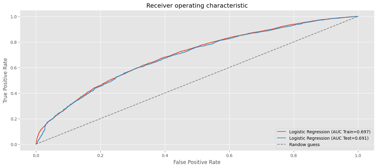
best_clf_rf = random_search.best_estimator_
print(f"Best hyperparameters RandomizedSearchCV:\n")
pprint(random_search.best_params_)

# AUC en train.
fpr, tpr, _ = roc_curve(y_train, best_clf_rf.predict_proba(X_train)[:, 1])
roc_auc = auc(fpr,tpr)
plt.plot(fpr, tpr, label=f"Logistic Regression (AUC Train={roc_auc:.3f})")

# AUC en test.
fpr, tpr, _ = roc_curve(y_test, best_clf_rf.predict_proba(X_test)[:, 1])
roc_auc = auc(fpr,tpr)
plt.plot(fpr, tpr, label=f"Logistic Regression (AUC Test={roc_auc:.3f})")

plt.xlabel("False Positive Rate")
plt.ylabel("True Positive Rate")
plt.title("Receiver operating characteristic")
plt.plot((0,1), (0,1), ls="--", color="grey", label="Randow guess")
plt.legend(loc="lower right")
plt.show()

Best hyperparameters RandomizedSearchCV:

{'classifier__class_weight': None,
 'classifier__max_depth': 6,
 'classifier__max_features': 'sqrt',
 'classifier__min_samples_leaf': 8,
 'classifier__min_samples_split': 200,
 'classifier__n_estimators': 300}

pd.DataFrame(random_search.cv_results_).sort_values("rank_test_score")

	mean_fit_time	std_fit_time	mean_score_time	std_score_time	param_classifier__n_estimators	param_classifier__min_samples_split	param_classifier__min_samples_leaf	param_classifier__max_features	param_classifier__max_depth	param_classifier__class_weight	...	mean_test_score	std_test_score	rank_test_score	split0_train_score	split1_train_score	split2_train_score	split3_train_score	split4_train_score	mean_train_score	std_train_score
16	16.120745	0.756754	0.451684	0.049141	300	200	8	sqrt	6	None	...	0.684039	0.010981	1	0.697580	0.703678	0.696113	0.699628	0.700399	0.699479	0.002586
0	12.641539	0.606206	0.386319	0.044912	300	400	4	log2	6	balanced	...	0.683863	0.011024	2	0.694940	0.700450	0.692768	0.696293	0.697424	0.696375	0.002561
29	12.706938	0.363876	0.430411	0.088084	300	400	8	log2	6	None	...	0.683502	0.010245	3	0.695165	0.700377	0.692794	0.696415	0.696551	0.696260	0.002460
42	15.361053	0.360445	0.481432	0.098843	300	300	4	sqrt	6	balanced	...	0.683237	0.011474	4	0.696085	0.702120	0.694693	0.698762	0.698904	0.698113	0.002566
34	8.534808	0.452824	0.290133	0.048471	200	200	2	sqrt	5	None	...	0.682859	0.011200	5	0.693568	0.697365	0.690215	0.693960	0.694769	0.693975	0.002299
35	4.329882	0.384941	0.177673	0.025607	100	400	8	log2	6	None	...	0.682825	0.010329	6	0.693750	0.699881	0.692396	0.695537	0.695518	0.695416	0.002524
7	20.883098	2.392378	0.576285	0.045558	500	350	2	sqrt	5	balanced	...	0.682535	0.011183	7	0.691745	0.697505	0.689118	0.692871	0.693922	0.693032	0.002750
5	2.739533	0.234485	0.133403	0.042839	50	200	8	sqrt	6	balanced	...	0.682533	0.010942	8	0.695563	0.703438	0.695088	0.701147	0.700154	0.699078	0.003247
27	2.237976	0.183861	0.138870	0.055458	50	350	4	log2	6	None	...	0.682242	0.011230	9	0.694072	0.700296	0.692561	0.697746	0.696477	0.696230	0.002721
8	4.376231	0.256418	0.183316	0.053242	100	350	8	sqrt	5	None	...	0.682233	0.011151	10	0.691473	0.696697	0.690045	0.691742	0.693273	0.692646	0.002270
30	2.073558	0.239400	0.117784	0.021059	50	350	4	sqrt	5	None	...	0.682171	0.011629	11	0.691399	0.696251	0.689745	0.692414	0.692223	0.692407	0.002141
36	7.533586	0.501849	0.257335	0.031852	200	300	2	log2	5	None	...	0.682092	0.010704	12	0.691000	0.696646	0.688540	0.693092	0.694178	0.692691	0.002760
19	10.962007	0.574778	0.358688	0.027562	300	200	2	log2	5	None	...	0.681950	0.010883	13	0.692178	0.697177	0.689187	0.692952	0.694574	0.693213	0.002642
20	2.103668	0.317394	0.098545	0.011505	50	200	4	sqrt	5	None	...	0.681674	0.011001	14	0.691145	0.699600	0.689926	0.694043	0.694541	0.693851	0.003355
3	17.626674	1.342634	0.574237	0.041517	500	400	2	log2	5	None	...	0.681604	0.010878	15	0.690463	0.695424	0.687813	0.692265	0.693044	0.691802	0.002553
9	1.826581	0.098950	0.118395	0.031796	50	400	2	sqrt	4	balanced	...	0.681194	0.011579	16	0.686941	0.691974	0.684690	0.688937	0.686513	0.687811	0.002481
40	2.161657	0.334028	0.121646	0.029652	50	300	8	log2	5	balanced	...	0.681050	0.011138	17	0.691714	0.696238	0.686335	0.690643	0.690556	0.691097	0.003162
14	1.863539	0.276670	0.119617	0.041825	50	200	2	sqrt	4	None	...	0.680969	0.010322	18	0.688415	0.691194	0.684241	0.688602	0.688684	0.688227	0.002239
31	10.432647	1.122015	0.457679	0.128345	300	350	8	sqrt	4	balanced	...	0.680895	0.011153	19	0.686858	0.692583	0.684766	0.688114	0.688167	0.688097	0.002560
1	1.505686	0.131261	0.110669	0.030812	50	300	4	sqrt	4	balanced	...	0.680803	0.011272	20	0.687101	0.690594	0.683461	0.689091	0.688071	0.687663	0.002399
13	16.498600	0.812424	0.595335	0.093352	500	300	2	sqrt	4	balanced	...	0.680798	0.010905	21	0.687358	0.693331	0.684472	0.688970	0.689715	0.688769	0.002905
23	15.395073	0.977171	0.593261	0.134874	500	200	8	log2	4	None	...	0.680558	0.011216	22	0.687835	0.692031	0.684742	0.687239	0.689570	0.688283	0.002430
49	7.026132	0.405267	0.179307	0.012492	300	200	2	sqrt	4	None	...	0.680522	0.011565	23	0.687683	0.692717	0.685569	0.689119	0.688933	0.688804	0.002330
46	14.167139	0.537839	0.532594	0.062210	500	350	8	log2	4	None	...	0.680323	0.010919	24	0.686655	0.691613	0.683935	0.687450	0.688825	0.687695	0.002526
6	9.469868	0.353936	0.329408	0.060259	300	200	4	log2	4	None	...	0.680212	0.011509	25	0.686565	0.691973	0.685289	0.688355	0.689350	0.688307	0.002310
25	7.190473	0.805285	0.244394	0.048460	200	400	4	sqrt	4	None	...	0.680163	0.011220	26	0.686478	0.691110	0.683665	0.687951	0.688443	0.687529	0.002444
28	8.738867	0.498346	0.328832	0.024704	300	400	8	log2	4	None	...	0.680093	0.010814	27	0.686108	0.690232	0.683810	0.686899	0.688897	0.687189	0.002229
38	3.532913	0.484375	0.178086	0.040821	100	200	4	log2	4	None	...	0.679920	0.010469	28	0.687113	0.691749	0.684868	0.687074	0.689432	0.688047	0.002347
17	1.539486	0.206834	0.108952	0.020393	50	300	8	sqrt	3	balanced	...	0.679642	0.010943	29	0.685590	0.689247	0.680827	0.684855	0.683024	0.684709	0.002803
45	6.057740	0.134378	0.291595	0.064903	200	200	8	log2	4	None	...	0.679593	0.011658	30	0.686323	0.690985	0.684919	0.687381	0.688379	0.687597	0.002046
43	1.514015	0.296282	0.093716	0.011299	50	400	8	log2	4	None	...	0.679164	0.010390	31	0.689204	0.691818	0.681386	0.686454	0.688740	0.687520	0.003509
44	1.650851	0.111136	0.096380	0.014254	50	350	8	log2	4	balanced	...	0.679006	0.009414	32	0.687403	0.691714	0.683418	0.685986	0.688036	0.687311	0.002714
33	5.131035	0.328847	0.228705	0.018288	200	300	2	sqrt	3	balanced	...	0.678841	0.010733	33	0.683792	0.689312	0.679600	0.683706	0.684785	0.684239	0.003100
18	6.811473	0.641759	0.314990	0.052629	300	400	8	log2	3	balanced	...	0.678505	0.010788	34	0.683745	0.689870	0.680317	0.682271	0.683527	0.683946	0.003203
15	1.533135	0.273691	0.095058	0.005039	50	350	8	sqrt	3	None	...	0.677466	0.011033	35	0.680935	0.685483	0.678103	0.683690	0.683037	0.682250	0.002533
26	4.145530	0.471337	0.215849	0.039624	200	400	2	log2	2	balanced	...	0.676829	0.011165	36	0.679048	0.684004	0.675850	0.681361	0.682733	0.680599	0.002887
39	4.117847	0.284574	0.175442	0.013987	200	350	8	sqrt	2	balanced	...	0.676762	0.010851	37	0.679234	0.683862	0.676359	0.678387	0.680427	0.679654	0.002488
32	4.305047	0.395058	0.165247	0.010751	200	350	4	log2	2	balanced	...	0.676508	0.010077	38	0.677898	0.685620	0.676430	0.678297	0.681794	0.680008	0.003313
22	2.116478	0.333756	0.124019	0.025196	100	400	2	log2	2	balanced	...	0.676491	0.010230	39	0.679777	0.686171	0.674982	0.678476	0.680000	0.679881	0.003621
21	10.553237	0.798287	0.431662	0.114725	500	300	2	sqrt	2	balanced	...	0.676438	0.010271	40	0.679693	0.685091	0.676375	0.679722	0.680221	0.680220	0.002794
10	1.524576	0.281466	0.081630	0.002134	50	200	8	log2	3	balanced	...	0.675832	0.010624	41	0.680786	0.689075	0.678871	0.682642	0.683066	0.682888	0.003433
2	1.971639	0.187856	0.107794	0.008805	100	200	8	log2	2	None	...	0.675504	0.010425	42	0.679291	0.683818	0.675425	0.678325	0.679784	0.679329	0.002706
41	4.230253	0.275220	0.171049	0.026982	200	300	8	log2	2	None	...	0.675364	0.010568	43	0.679145	0.682780	0.673849	0.679605	0.681610	0.679398	0.003073
24	9.876326	0.686199	0.340800	0.020144	500	300	8	log2	2	None	...	0.675223	0.010587	44	0.677987	0.683247	0.674950	0.677599	0.679244	0.678605	0.002710
47	6.882808	1.090894	0.310430	0.062984	300	200	4	sqrt	2	None	...	0.675189	0.010153	45	0.678632	0.684270	0.675258	0.677125	0.679915	0.679040	0.003042
48	5.753073	0.314057	0.189903	0.043841	300	200	8	sqrt	2	None	...	0.675164	0.011016	46	0.678695	0.683297	0.675967	0.677613	0.678123	0.678739	0.002454
11	10.939743	0.819781	0.414020	0.048205	500	200	8	sqrt	2	None	...	0.674908	0.011137	47	0.678704	0.683048	0.675636	0.676852	0.677795	0.678407	0.002534
12	10.483544	0.628677	0.531626	0.143267	500	300	8	sqrt	2	None	...	0.674789	0.010587	48	0.677970	0.683088	0.675379	0.677620	0.679142	0.678640	0.002536
4	6.552659	0.890362	0.261461	0.043635	300	400	8	sqrt	2	None	...	0.674400	0.011429	49	0.677713	0.681223	0.674751	0.677710	0.679371	0.678154	0.002139
37	1.073801	0.030192	0.084940	0.009541	50	350	2	log2	2	None	...	0.673607	0.009648	50	0.679291	0.683190	0.671352	0.676714	0.678831	0.677876	0.003875

50 rows × 26 columns

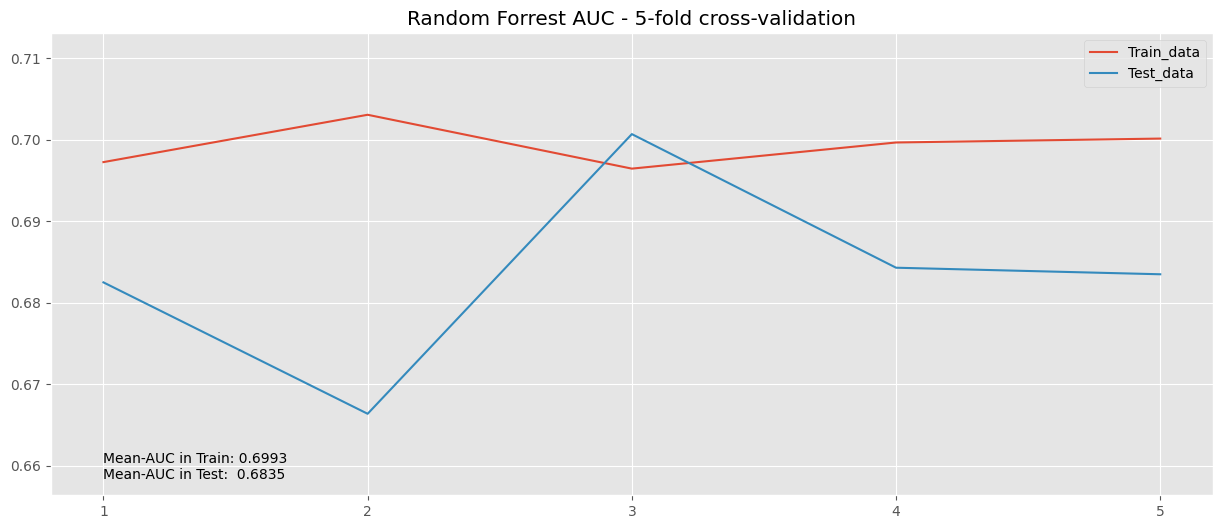
cv_results_rf_final = cross_validate(
    best_clf_rf, X_train, y_train, cv=5,
    scoring=("roc_auc", "accuracy"),
    return_train_score=True
)

train_lr, test_lr = cv_results_rf_final["train_roc_auc"], cv_results_rf_final["test_roc_auc"]

values_aucs_lr = np.concatenate((train_lr, test_lr), axis=None)
min_y, max_y = values_aucs_lr.min() -0.01 , values_aucs_lr.max()+ 0.01
means_rf = (train_lr.mean(), test_lr.mean())
##
plt.plot(cv_results_rf_final["train_roc_auc"], label="Train_data")
plt.plot(cv_results_rf_final["test_roc_auc"], label="Test_data")
plt.title("Random Forrest AUC - 5-fold cross-validation")
plt.legend()
plt.text(0, min_y + 4e-03, f"Mean-AUC in Train: {means_rf[0]:.4f}")
plt.text(0, min_y + 2e-03, f"Mean-AUC in Test:  {means_rf[1]:.4f}")
plt.ylim(min_y, max_y)
plt.xticks(np.arange(0,5), np.arange(1,6))
plt.show()