Analisis descriptivo multivariado.

Universidad Central

Maestría en analítica de datos

Métodos estadísticos para analítica de datos.

Docente: Luis Andrés Campos Maldonado.

import warnings
warnings.filterwarnings("ignore")

import pandas as pd
import numpy as np
import matplotlib.pyplot as plt
import seaborn as sns
import plotly.express as px
##
sns.set_theme()

Cereal

Vamos a cargar la base de datos de Cereal, que contiene información nutricional de diferentes marcas de cereales.

url = "https://raw.githubusercontent.com/lacamposm/Metodos_Estadisticos/main/data/Cereal.csv"
df = pd.read_csv(url, sep=";", decimal=",", index_col=0)
df.head()

	Fabrica	Calorias	Proteina	Grasa	Sodio	Fibra	Carbohidratos	Azucares	Potasio	Vitaminas
Cereal
100% Bran	N	212.12121	12.121212	3.030303	393.93939	30.303030	15.15152	18.181818	848.48485	enriched
All-Bran	K	212.12121	12.121212	3.030303	787.87879	27.272727	21.21212	15.151515	969.69697	enriched
All-Bran with Extra Fiber	K	100.00000	8.000000	0.000000	280.00000	28.000000	16.00000	0.000000	660.00000	enriched
Apple Cinnamon Cheerios	G	146.66667	2.666667	2.666667	240.00000	2.000000	14.00000	13.333333	93.33333	enriched
Apple Jacks	K	110.00000	2.000000	0.000000	125.00000	1.000000	11.00000	14.000000	30.00000	enriched

Observamos los tipos de datos en cada una de las columna del DataFrame.

df.dtypes

Fabrica           object
Calorias         float64
Proteina         float64
Grasa            float64
Sodio            float64
Fibra            float64
Carbohidratos    float64
Azucares         float64
Potasio          float64
Vitaminas         object
dtype: object

Con el método select_dtypes() podemos obtener las columnas cuyos valores son numéricos.

df_numeric = df.select_dtypes(np.number)
df_numeric

	Calorias	Proteina	Grasa	Sodio	Fibra	Carbohidratos	Azucares	Potasio
Cereal
100% Bran	212.12121	12.121212	3.030303	393.93939	30.303030	15.15152	18.181818	848.48485
All-Bran	212.12121	12.121212	3.030303	787.87879	27.272727	21.21212	15.151515	969.69697
All-Bran with Extra Fiber	100.00000	8.000000	0.000000	280.00000	28.000000	16.00000	0.000000	660.00000
Apple Cinnamon Cheerios	146.66667	2.666667	2.666667	240.00000	2.000000	14.00000	13.333333	93.33333
Apple Jacks	110.00000	2.000000	0.000000	125.00000	1.000000	11.00000	14.000000	30.00000
...	...	...	...	...	...	...	...	...
Triples	146.66667	2.666667	1.333333	333.33333	0.000000	28.00000	4.000000	80.00000
Trix	110.00000	1.000000	1.000000	140.00000	0.000000	13.00000	12.000000	25.00000
Wheat Chex	149.25373	4.477612	1.492537	343.28358	4.477612	25.37313	4.477612	171.64179
Wheaties	100.00000	3.000000	1.000000	200.00000	3.000000	17.00000	3.000000	110.00000
Wheaties Honey Gold	146.66667	2.666667	1.333333	266.66667	1.333333	21.33333	10.666667	80.00000

65 rows × 8 columns

## Así mismo con las columnas de tipo "object"
df_object = df.select_dtypes(include=["object"])
df_object

	Fabrica	Vitaminas
Cereal
100% Bran	N	enriched
All-Bran	K	enriched
All-Bran with Extra Fiber	K	enriched
Apple Cinnamon Cheerios	G	enriched
Apple Jacks	K	enriched
...	...	...
Triples	G	enriched
Trix	G	enriched
Wheat Chex	R	enriched
Wheaties	G	enriched
Wheaties Honey Gold	G	enriched

65 rows × 2 columns

Vamos a recoger en un lista los nombres de las columnas que son de tipo “numerico”.

Ejercicio 1.

En un lista ubique todos los nombre de las columnas que son de tipo “numerico”. Piense en que el numéro de features podría ser banstante grande.

Respuesta:

## Celda de código para probar.
features_numeric = [feature for feature in df_numeric.columns]
features_numeric

['Calorias',
 'Proteina',
 'Grasa',
 'Sodio',
 'Fibra',
 'Carbohidratos',
 'Azucares',
 'Potasio']

Así mismo lo podemos hacer para las no numéricas.

Ejercicio 2.

Solucione el mismo problema que en el Ejercicio 1 pero con las varibles de tipo “object”.

Respuesta:

## Celda de código para probar.
features_categories = [feature for feature in df_object.columns]
features_categories

['Fabrica', 'Vitaminas']

Matriz de covarianzas y de correlación.

Cuando se tiene un conjunto de variables cuantitativas, por cada par de ellas se calcula la covarianza:

\[Cov(X,Y)=\frac{1}{n-1}\sum_{i=1}^n (X_i-\bar{X})(Y_i-\bar{Y})\]

Estos valores conformarán la matriz de covarianzas. El coeficiente de correlación lineal se define como:

\[\rho_{XY}=\frac{Cov(X;Y)}{sd(X)sd(Y)}\]

## Matriz de varianzas-covarianzas
df_numeric.cov()

	Calorias	Proteina	Grasa	Sodio	Fibra	Carbohidratos	Azucares	Potasio
Calorias	3895.242099	116.442850	60.674383	4310.041188	148.608725	416.865952	180.380317	5362.723526
Proteina	116.442850	6.983432	1.790252	197.706130	13.122839	12.243296	2.850421	401.040187
Grasa	60.674383	1.790252	2.713399	55.851817	2.284043	2.550715	3.995474	96.005854
Sodio	4310.041188	197.706130	55.851817	17064.098428	396.983157	468.557877	161.021552	13109.507474
Fibra	148.608725	13.122839	2.284043	396.983157	37.618644	10.547819	5.329678	1065.826587
Carbohidratos	416.865952	12.243296	2.550715	468.557877	10.547819	71.714955	-2.017438	369.551907
Azucares	180.380317	2.850421	3.995474	161.021552	5.329678	-2.017438	34.050018	285.976158
Potasio	5362.723526	401.040187	96.005854	13109.507474	1065.826587	369.551907	285.976158	32503.973299

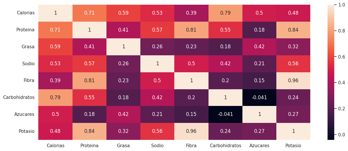
### Matriz de correlación lineal de pearson
df_numeric.corr().round(4)

	Calorias	Proteina	Grasa	Sodio	Fibra	Carbohidratos	Azucares	Potasio
Calorias	1.0000	0.7060	0.5902	0.5287	0.3882	0.7887	0.4953	0.4766
Proteina	0.7060	1.0000	0.4113	0.5727	0.8096	0.5471	0.1848	0.8418
Grasa	0.5902	0.4113	1.0000	0.2596	0.2261	0.1829	0.4157	0.3233
Sodio	0.5287	0.5727	0.2596	1.0000	0.4955	0.4236	0.2112	0.5566
Fibra	0.3882	0.8096	0.2261	0.4955	1.0000	0.2031	0.1489	0.9639
Carbohidratos	0.7887	0.5471	0.1829	0.4236	0.2031	1.0000	-0.0408	0.2420
Azucares	0.4953	0.1848	0.4157	0.2112	0.1489	-0.0408	1.0000	0.2718
Potasio	0.4766	0.8418	0.3233	0.5566	0.9639	0.2420	0.2718	1.0000

La matriz anterior muestra la relación lineal entre cada par de variables, por su supuesto en la diagonal principal tenemos la correlación de la variable con ella misma, es decir 1.

Ejercicio 3.

Haga uso de plotly_express para construir un scatter plot de las siguientes variables:

• Potasio vs. Fibra

## Celda de código para probra.
## Grafico de fibra y potasio.
fig = px.scatter(df_numeric, x = df_numeric.Potasio, y = df_numeric.Fibra)
fig.show()

La relación de las variables anteriores muestra que al parecer a mayor contenido de Potasio se incrementa la fibra.

Ejercicio 4.

Obtenga el valor de esta correlación haciendo uso de código.

Respuesta:

## Celda de código para probar.
corr = df_numeric.corr().round(4).loc["Fibra","Potasio"]
print("La correlación de la variable Fibra y la variable Potasio es {:.3f}".format(corr))

La correlación de la variable Fibra y la variable Potasio es 0.964

Recuerde que muchas veces un plot dice más que mil palabras… Veamos la matriz de correlación con un mapa de calor

## Mapa de calor de la matriz de correlación.
plt.figure(figsize=(15,6))
sns.heatmap(df_numeric.corr(), annot=True)
plt.show()

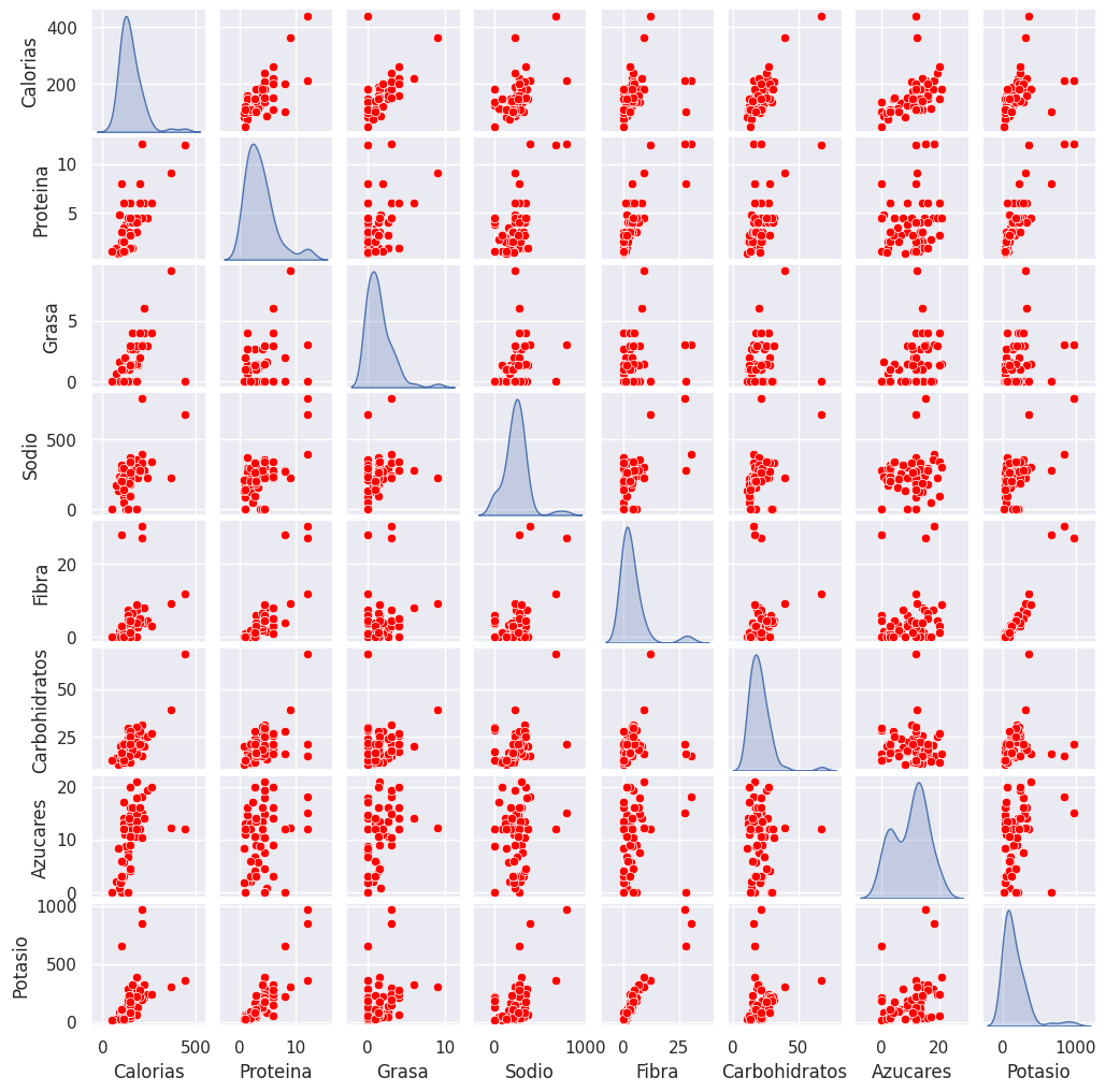
Diagramas de dispersión

El diagrama de dispersión sirve para visualizar relaciones entre un par de variables cuantitativas.

Ejercicio 5.

Construya un pairplot de todas las variables numéricas en el conjunto de datos, y la diagonal presente un kde-plot.

Respuesta:

## Celda de código para probar.
g = sns.pairplot(df_numeric, palette="dark", diag_kind="kde", plot_kws={"color":"red"})
g.fig.set_size_inches(10,10)

Un plot más dinámico incluyendo el nombre del cereal lo podemos ver con el siguiente código:

## Scatter plot entre Carbohidratos y Azucares. use hover_name = df.index
## Complete el siguiente código
## fig = px.?????(df, x = ???? , y = ????, ?????=?????)
## ???.show()

Replique los mismos gráficos mostrando un scatter-plot de:

• Potasio vs. Sodio

• Proteina vs. Fibra

## Celda de código para probar.
fig = px.scatter(df, x = "Potasio", y = "Sodio", hover_name = df.index)
fig.show()

## Celda de código para probar.
fig = px.scatter(df, x = "Proteina", y = "Fibra", hover_name = df.index)
fig.show()

Tablas de contingencia.

Vamos a hacer uso de pd.crosstab() para construir una tabla de contingencia, recordando que dicha tabla contiene los conteos de una o más variables cualitativas.

url="https://raw.githubusercontent.com/lacamposm/Metodos_Estadisticos/main/data/PruebaSaber1.csv"
df_icfes1 = pd.read_csv(url, sep=";", encoding="latin1",low_memory=False)
df_icfes1.shape

(10000, 78)

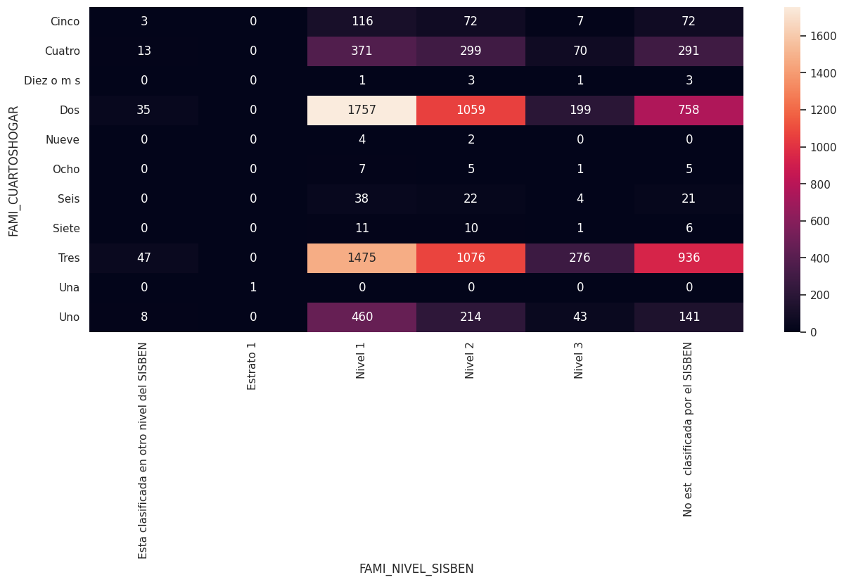
crosstab = pd.crosstab(df_icfes1["FAMI_CUARTOSHOGAR"], df_icfes1["FAMI_NIVEL_SISBEN"])
crosstab

FAMI_NIVEL_SISBEN	Esta clasificada en otro nivel del SISBEN	Estrato 1	Nivel 1	Nivel 2	Nivel 3	No est  clasificada por el SISBEN
FAMI_CUARTOSHOGAR
Cinco	3	0	116	72	7	72
Cuatro	13	0	371	299	70	291
Diez o m s	0	0	1	3	1	3
Dos	35	0	1757	1059	199	758
Nueve	0	0	4	2	0	0
Ocho	0	0	7	5	1	5
Seis	0	0	38	22	4	21
Siete	0	0	11	10	1	6
Tres	47	0	1475	1076	276	936
Una	0	1	0	0	0	0
Uno	8	0	460	214	43	141

plt.figure(figsize=(15,6))
sns.heatmap(crosstab, annot=True,fmt=".0f")
plt.show()

Ejercicio 5.

¿Que puede comentar del mapa de calor anterior?

Respuesta

Otros gráficos multivariados.

df_group = df_icfes1.groupby(["FAMI_CUARTOSHOGAR", "FAMI_NIVEL_SISBEN"]).size()
df_group

FAMI_CUARTOSHOGAR  FAMI_NIVEL_SISBEN                        
Cinco              Esta clasificada en otro nivel del SISBEN       3
                   Nivel 1                                       116
                   Nivel 2                                        72
                   Nivel 3                                         7
                   No est  clasificada por el SISBEN              72
Cuatro             Esta clasificada en otro nivel del SISBEN      13
                   Nivel 1                                       371
                   Nivel 2                                       299
                   Nivel 3                                        70
                   No est  clasificada por el SISBEN             291
Diez o m s         Nivel 1                                         1
                   Nivel 2                                         3
                   Nivel 3                                         1
                   No est  clasificada por el SISBEN               3
Dos                Esta clasificada en otro nivel del SISBEN      35
                   Nivel 1                                      1757
                   Nivel 2                                      1059
                   Nivel 3                                       199
                   No est  clasificada por el SISBEN             758
Nueve              Nivel 1                                         4
                   Nivel 2                                         2
Ocho               Nivel 1                                         7
                   Nivel 2                                         5
                   Nivel 3                                         1
                   No est  clasificada por el SISBEN               5
Seis               Nivel 1                                        38
                   Nivel 2                                        22
                   Nivel 3                                         4
                   No est  clasificada por el SISBEN              21
Siete              Nivel 1                                        11
                   Nivel 2                                        10
                   Nivel 3                                         1
                   No est  clasificada por el SISBEN               6
Tres               Esta clasificada en otro nivel del SISBEN      47
                   Nivel 1                                      1475
                   Nivel 2                                      1076
                   Nivel 3                                       276
                   No est  clasificada por el SISBEN             936
Una                Estrato 1                                       1
Uno                Esta clasificada en otro nivel del SISBEN       8
                   Nivel 1                                       460
                   Nivel 2                                       214
                   Nivel 3                                        43
                   No est  clasificada por el SISBEN             141
dtype: int64

df_group = df_icfes1.groupby(["FAMI_CUARTOSHOGAR", "FAMI_NIVEL_SISBEN"]).size()
df_group = df_group.reset_index(name="Conteo",)
df_group

	FAMI_CUARTOSHOGAR	FAMI_NIVEL_SISBEN	Conteo
0	Cinco	Esta clasificada en otro nivel del SISBEN	3
1	Cinco	Nivel 1	116
2	Cinco	Nivel 2	72
3	Cinco	Nivel 3	7
4	Cinco	No est  clasificada por el SISBEN	72
5	Cuatro	Esta clasificada en otro nivel del SISBEN	13
6	Cuatro	Nivel 1	371
7	Cuatro	Nivel 2	299
8	Cuatro	Nivel 3	70
9	Cuatro	No est  clasificada por el SISBEN	291
10	Diez o m s	Nivel 1	1
11	Diez o m s	Nivel 2	3
12	Diez o m s	Nivel 3	1
13	Diez o m s	No est  clasificada por el SISBEN	3
14	Dos	Esta clasificada en otro nivel del SISBEN	35
15	Dos	Nivel 1	1757
16	Dos	Nivel 2	1059
17	Dos	Nivel 3	199
18	Dos	No est  clasificada por el SISBEN	758
19	Nueve	Nivel 1	4
20	Nueve	Nivel 2	2
21	Ocho	Nivel 1	7
22	Ocho	Nivel 2	5
23	Ocho	Nivel 3	1
24	Ocho	No est  clasificada por el SISBEN	5
25	Seis	Nivel 1	38
26	Seis	Nivel 2	22
27	Seis	Nivel 3	4
28	Seis	No est  clasificada por el SISBEN	21
29	Siete	Nivel 1	11
30	Siete	Nivel 2	10
31	Siete	Nivel 3	1
32	Siete	No est  clasificada por el SISBEN	6
33	Tres	Esta clasificada en otro nivel del SISBEN	47
34	Tres	Nivel 1	1475
35	Tres	Nivel 2	1076
36	Tres	Nivel 3	276
37	Tres	No est  clasificada por el SISBEN	936
38	Una	Estrato 1	1
39	Uno	Esta clasificada en otro nivel del SISBEN	8
40	Uno	Nivel 1	460
41	Uno	Nivel 2	214
42	Uno	Nivel 3	43
43	Uno	No est  clasificada por el SISBEN	141

fig = px.bar(df_group, x="FAMI_CUARTOSHOGAR", y="Conteo", color="FAMI_NIVEL_SISBEN")
fig.show()

Ejercicio 6.

¿Observa lo mismo que en el mapa de calor, o quizá se observa información no percibida antes?

Respuesta:

En el repositorio de Github, tenemos más tablas de resultados del ICFES, vamos a importarlas todas y formar un único pandas DataFrame.

Ejercicio 7.

Construya el pd.DataFrame solicitado en el párrafo anterior. Llame este DataFrame df_icfes.

# Celda de código para probar.
url_main = "https://raw.githubusercontent.com/lacamposm/Metodos_Estadisticos/main/data/PruebaSaber"
#
df_icfes = pd.DataFrame()
for i in range(1, 13):
  url = url_main + str(i) + ".csv"
  df_temp = pd.read_csv(url, sep=";", encoding="latin1", low_memory=False)
  print(url," Shape:",df_temp.shape)
  df_icfes = pd.concat([df_icfes, df_temp])

print("\nEl tamaño del Dataframe resultante es: {}".format(df_icfes.shape))

https://raw.githubusercontent.com/lacamposm/Metodos_Estadisticos/main/data/PruebaSaber1.csv  Shape: (10000, 78)

https://raw.githubusercontent.com/lacamposm/Metodos_Estadisticos/main/data/PruebaSaber2.csv  Shape: (10000, 78)

https://raw.githubusercontent.com/lacamposm/Metodos_Estadisticos/main/data/PruebaSaber3.csv  Shape: (10000, 78)

https://raw.githubusercontent.com/lacamposm/Metodos_Estadisticos/main/data/PruebaSaber4.csv  Shape: (10000, 78)

https://raw.githubusercontent.com/lacamposm/Metodos_Estadisticos/main/data/PruebaSaber5.csv  Shape: (10000, 78)

https://raw.githubusercontent.com/lacamposm/Metodos_Estadisticos/main/data/PruebaSaber6.csv  Shape: (10000, 78)

https://raw.githubusercontent.com/lacamposm/Metodos_Estadisticos/main/data/PruebaSaber7.csv  Shape: (10000, 78)

https://raw.githubusercontent.com/lacamposm/Metodos_Estadisticos/main/data/PruebaSaber8.csv  Shape: (10000, 78)

https://raw.githubusercontent.com/lacamposm/Metodos_Estadisticos/main/data/PruebaSaber9.csv  Shape: (10000, 78)

https://raw.githubusercontent.com/lacamposm/Metodos_Estadisticos/main/data/PruebaSaber10.csv  Shape: (10000, 78)

https://raw.githubusercontent.com/lacamposm/Metodos_Estadisticos/main/data/PruebaSaber11.csv  Shape: (10000, 78)

https://raw.githubusercontent.com/lacamposm/Metodos_Estadisticos/main/data/PruebaSaber12.csv  Shape: (2504, 78)

El tamaño del Dataframe resultante es: (112504, 78)

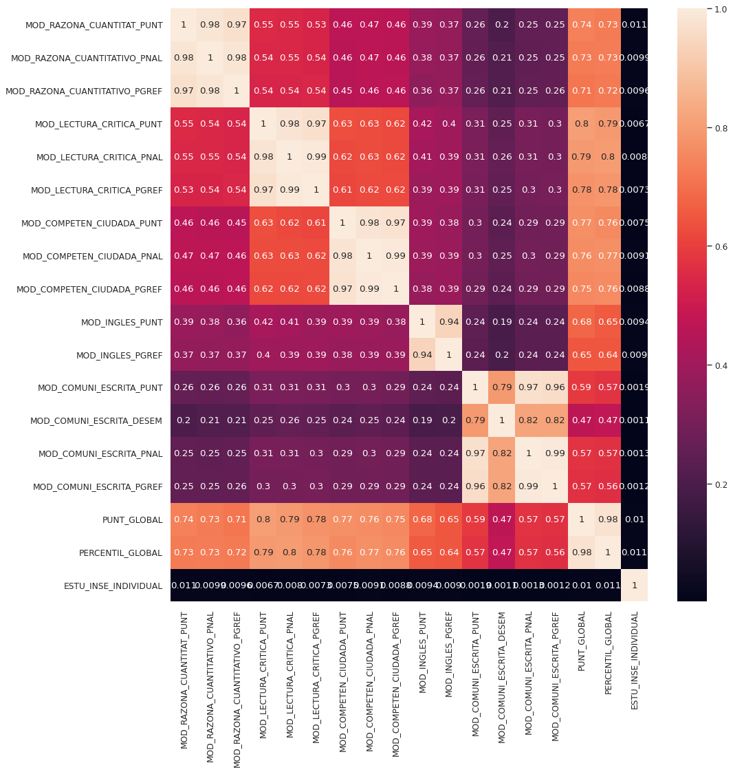
corre = df_icfes.select_dtypes(np.number).corr()
plt.figure(figsize=(14, 14), dpi=80)
sns.heatmap(corre,annot=True )
plt.show()

px.scatter(
    data_frame=df_icfes,
    x="MOD_LECTURA_CRITICA_PUNT",
    y="PUNT_GLOBAL",
    title="Scatter-plot: Puntaje Lectura crítica y Puntaje global"
).show()

Ejercicio 8.

Construya con plotly_express un bar plot del conteo de elementos del cruce entre las variables FAMI_CUARTOSHOGAR y FAMI_NIVEL_SISBEN. En el eje \(x\) debe estar la varible FAMI_CUARTOSHOGAR mientras que en el eje \(y\) el conteo y distinguible por la variable FAMI_NIVEL_SISBEN.

Hint: Use el parámetro color="FAMI_NIVEL_SISBEN"

df_group1 = df_icfes.groupby(["FAMI_CUARTOSHOGAR", "FAMI_NIVEL_SISBEN"]).size()
df_group1 = df_group1.reset_index(name="Conteo")

px.bar(
    df_group1,
    x="FAMI_CUARTOSHOGAR",
    y="Conteo",
    color="FAMI_NIVEL_SISBEN"
).show()

px.scatter(
    df_icfes,
    x="MOD_RAZONA_CUANTITAT_PUNT",
    y="MOD_LECTURA_CRITICA_PUNT"
).show()

Vamos a considerar el DataFrame de las medias para los distintos grupos al cruzar las variables género del estudiante (ESTU_GENERO) y el departamento (ESTU_INST_DEPARTAMENTO)

df_group2 = df_icfes.groupby(["ESTU_GENERO", "ESTU_INST_DEPARTAMENTO"])[
    df_icfes.select_dtypes(np.number).columns
].mean()

df_group2 = df_group2.reset_index()
df_group2

	ESTU_GENERO	ESTU_INST_DEPARTAMENTO	MOD_RAZONA_CUANTITAT_PUNT	MOD_RAZONA_CUANTITATIVO_PNAL	MOD_RAZONA_CUANTITATIVO_PGREF	MOD_LECTURA_CRITICA_PUNT	MOD_LECTURA_CRITICA_PNAL	MOD_LECTURA_CRITICA_PGREF	MOD_COMPETEN_CIUDADA_PUNT	MOD_COMPETEN_CIUDADA_PNAL	MOD_COMPETEN_CIUDADA_PGREF	MOD_INGLES_PUNT	MOD_INGLES_PGREF	MOD_COMUNI_ESCRITA_PUNT	MOD_COMUNI_ESCRITA_DESEM	MOD_COMUNI_ESCRITA_PNAL	MOD_COMUNI_ESCRITA_PGREF	PUNT_GLOBAL	PERCENTIL_GLOBAL	ESTU_INSE_INDIVIDUAL
0	F	ANTIOQUIA	101.772414	53.034943	54.268046	105.693333	58.797241	58.834483	103.767356	55.794943	55.534713	102.144368	54.313103	106.400924	2.760739	59.833718	59.248961	103.862529	58.614713	100.549658
1	F	ATLANTICO	96.815789	45.671053	47.680099	99.495066	49.660362	50.739309	98.804276	48.567434	49.110197	100.341283	53.285362	100.752902	2.466003	51.095357	49.945274	99.069079	48.935033	133.363980
2	F	BOGOTA	96.969663	45.931150	46.851030	99.762009	50.002411	50.006228	100.119699	50.410588	50.068408	97.818383	48.282069	101.404134	2.529434	52.469595	51.670651	99.081668	49.123154	81.417541
3	F	BOGOTµ, D.C.	11.000000	109.000000	66.000000	69.000000	129.000000	92.000000	93.000000	107.000000	62.000000	61.000000	66.000000	68.000000	118.000000	3.000000	82.000000	80.000000	114.000000	84.000000
4	F	BOLIVAR	95.093143	43.630286	43.432571	99.786857	50.230857	49.936571	98.901714	48.574286	48.072571	100.458286	50.823429	101.436563	2.524221	52.294694	51.540946	98.965143	48.772000	86.990817
5	F	BOYACA	96.460432	44.863309	46.924460	100.881295	51.410072	52.410072	102.143885	53.428058	53.906475	92.208633	42.607914	104.211679	2.664234	56.029197	54.861314	98.881295	48.568345	48.749746
6	F	BUCARAMANGA	68.000000	103.000000	55.000000	58.000000	103.000000	57.000000	57.000000	90.000000	31.000000	29.000000	10.000000	10.000000	116.000000	3.000000	79.000000	78.000000	97.000000	44.000000
7	F	CALDAS	94.621415	42.338432	47.434034	97.403442	46.806883	52.315488	97.296367	46.191205	51.388145	95.642447	50.070746	103.402724	2.626459	55.324903	59.120623	97.311663	45.468451	45.701468
8	F	CAQUETA	106.714286	59.642857	59.500000	115.357143	68.000000	64.000000	110.785714	61.214286	55.785714	95.857143	44.785714	122.857143	3.571429	84.000000	80.071429	110.214286	68.214286	49.708245
9	F	CAUCA	96.644231	45.043269	45.197115	96.764423	45.423077	47.317308	98.538462	47.923077	50.307692	94.750000	45.076923	99.497585	2.454106	49.652174	51.903382	97.134615	45.317308	239.199711
10	F	CHOCO	102.500000	53.000000	49.000000	109.000000	66.000000	64.500000	110.000000	63.000000	62.500000	115.500000	75.500000	99.500000	2.500000	49.000000	51.500000	107.000000	62.000000	43.185549
11	F	CORDOBA	90.954545	36.909091	43.000000	93.136364	41.363636	43.454545	92.363636	38.772727	39.681818	88.818182	38.590909	97.090909	2.272727	44.000000	42.454545	92.500000	36.181818	45.198106
12	F	CUNDINAMARCA	105.243902	58.292683	54.829268	105.048780	57.073171	55.975610	103.121951	53.951220	54.000000	107.487805	58.048780	107.780488	2.780488	61.292683	62.682927	105.780488	62.682927	54.448160
13	F	HUILA	104.855072	58.289855	58.797101	105.086957	57.376812	58.478261	100.782609	51.057971	52.246377	102.927536	55.768116	108.608696	2.855072	63.710145	64.043478	104.507246	59.608696	47.899190
14	F	LA GUAJIRA	91.578947	39.017544	38.596491	90.421053	38.333333	39.877193	95.842105	44.578947	46.456140	88.929825	34.877193	96.910714	2.357143	46.696429	47.446429	92.438596	37.701754	44.642216
15	F	MAGDALENA	86.131387	30.133820	38.360097	90.416058	36.474453	40.982968	92.469586	38.880779	42.107056	86.520681	37.352798	96.606516	2.303258	45.293233	46.994987	89.863747	30.756691	44.257546
16	F	META	103.285714	56.000000	59.357143	104.642857	56.571429	54.785714	106.285714	59.000000	58.214286	103.285714	57.571429	101.923077	2.538462	52.153846	51.307692	102.428571	56.000000	51.887948
17	F	NARI¥O	99.586777	49.537190	53.636364	103.157025	55.520661	56.524793	101.123967	52.185950	52.706612	100.995868	55.111570	105.212500	2.695833	57.758333	57.408333	101.859504	55.276860	47.896739
18	F	NORTE SANTANDER	96.232353	45.014706	46.055882	96.329412	45.247059	45.270588	96.308824	45.238235	44.929412	92.811765	40.808824	101.339233	2.551622	52.572271	51.790560	96.538235	44.052941	141.779597
19	F	PUTUMAYO	98.586957	47.282609	46.326087	106.130435	58.304348	58.478261	107.086957	60.478261	61.173913	101.760870	53.717391	104.043478	2.608696	55.456522	56.804348	103.456522	56.543478	43.882931
20	F	QUINDIO	97.160000	46.091429	44.971429	97.920000	47.422857	45.314286	96.954286	45.988571	44.971429	103.771429	52.708571	105.988439	2.722543	59.028902	57.462428	100.148571	51.062857	55.444022
21	F	RISARALDA	102.338323	52.892216	53.224551	103.574850	54.964072	56.476048	103.188623	54.982036	56.697605	104.236527	58.479042	106.639640	2.774775	60.354354	62.684685	103.931138	57.278443	48.747086
22	F	SAN ANDRES	85.200000	28.300000	28.200000	97.900000	46.500000	47.000000	88.900000	35.300000	34.900000	121.700000	78.900000	102.888889	2.666667	56.222222	54.333333	97.300000	45.700000	48.792491
23	F	SANTANDER	102.139052	53.400639	53.045285	103.254129	54.831113	54.510922	102.790623	54.378796	53.924347	100.028237	50.905701	105.067878	2.699091	57.965794	57.605024	102.587640	55.923282	129.327564
24	F	SUCRE	84.000000	27.391304	31.956522	87.000000	31.782609	33.347826	87.739130	32.695652	33.391304	89.043478	39.260870	100.217391	2.521739	49.521739	49.043478	89.695652	28.869565	46.286020
25	F	TOLIMA	94.158831	41.922490	43.796696	96.062262	44.510801	46.048285	95.589581	44.176620	45.425667	92.886912	42.891995	98.982028	2.423620	49.218228	49.729140	95.331639	41.729352	228.120692
26	F	VALLE	100.744059	51.374771	52.452599	103.414381	55.513711	54.848930	101.316880	52.062157	51.798165	101.828763	52.672171	103.037585	2.617991	54.805299	54.018553	101.850701	54.382084	87.222468
27	M	ANTIOQUIA	109.816806	63.935804	62.572025	105.901879	58.693633	57.732777	104.268267	56.628392	56.127349	108.071503	58.626827	103.209424	2.604712	54.762304	55.265445	106.186326	62.670146	53.661166
28	M	ATLANTICO	101.709589	52.874886	52.311416	97.994521	47.587215	48.160731	96.626484	45.789954	46.510502	104.852968	57.042009	95.529248	2.246054	44.000000	44.220984	99.017352	49.296804	166.467902
29	M	BOGOTA	103.188834	54.833018	53.455043	99.886828	50.117522	49.752648	100.057469	50.483701	50.432245	101.509288	51.739701	97.743063	2.362631	47.108200	47.848990	100.289468	51.416560	98.756578
30	M	BOLIVAR	100.559278	51.036082	48.998711	96.900773	45.922036	45.236469	95.775129	44.567010	44.285438	101.637887	50.856959	95.801974	2.272368	44.223684	44.676974	97.750000	46.362758	91.415221
31	M	BOYACA	105.305085	58.186441	54.740113	100.734463	51.033898	51.141243	105.757062	58.378531	59.079096	96.853107	47.090395	100.171429	2.491429	50.754286	52.805714	101.536723	53.807910	48.400971
32	M	CALDAS	96.948370	46.103261	49.956522	94.605978	42.961957	47.573370	94.304348	42.581522	47.331522	95.516304	47.500000	97.754821	2.352617	46.911846	50.856749	95.576087	42.290761	192.208655
33	M	CALI	76.000000	97.000000	44.000000	47.000000	77.000000	13.000000	12.000000	92.000000	34.000000	33.000000	37.000000	38.000000	98.000000	2.000000	44.000000	41.000000	91.000000	28.000000
34	M	CAQUETA	94.000000	40.785714	38.500000	102.000000	52.285714	48.071429	98.642857	49.928571	46.785714	90.642857	33.714286	99.000000	2.357143	48.428571	44.928571	96.928571	43.357143	48.510087
35	M	CAUCA	99.751773	50.312057	48.773050	93.858156	42.063830	42.460993	93.588652	40.510638	41.971631	97.659574	46.134752	92.496403	2.172662	41.280576	42.848921	95.205674	41.553191	46.978423
36	M	CESAR	93.500000	44.000000	49.500000	90.500000	32.500000	44.000000	103.000000	54.500000	66.500000	98.500000	64.500000	96.000000	2.000000	46.000000	53.000000	96.000000	43.000000	50.954109
37	M	CHOCO	78.375000	21.000000	18.375000	74.250000	15.875000	15.500000	88.375000	30.125000	30.625000	89.625000	31.750000	72.000000	1.375000	17.500000	19.000000	80.500000	18.250000	47.082766
38	M	CORDOBA	105.916667	61.416667	68.416667	88.833333	35.166667	37.166667	88.833333	39.250000	40.333333	83.416667	30.416667	90.500000	1.833333	33.666667	31.833333	91.500000	33.500000	45.957908
39	M	CUNDINAMARCA	91.578740	38.652231	47.066929	89.620735	35.943570	45.872703	87.051181	32.517060	40.814961	96.337270	54.036745	90.784392	2.070106	37.916667	43.757937	90.950131	33.461942	178.863560
40	M	HUILA	106.775510	60.183673	59.775510	99.673469	49.755102	51.000000	98.653061	49.591837	50.775510	97.428571	50.551020	94.958333	2.291667	43.875000	46.208333	99.142857	49.816327	48.534396
41	M	LA GUAJIRA	97.774194	46.129032	44.064516	88.693548	34.032258	36.741935	88.790323	34.806452	38.016129	89.483871	35.645161	94.278689	2.213115	40.836066	43.278689	91.532258	33.870968	46.060031
42	M	MAGDALENA	90.629630	37.137566	45.312169	91.730159	38.148148	42.820106	93.111111	40.338624	43.783069	91.412698	44.084656	93.304813	2.128342	39.700535	41.112299	91.820106	34.936508	45.326718
43	M	META	100.666667	51.166667	48.833333	89.833333	32.000000	24.166667	100.166667	49.666667	44.500000	100.000000	39.000000	86.833333	1.500000	27.166667	26.500000	95.500000	40.833333	58.642623
44	M	NARI¥O	104.258427	56.247191	58.544944	100.640449	50.853933	52.415730	101.702247	51.994382	53.668539	102.471910	56.112360	100.610169	2.463277	50.468927	51.124294	101.825843	54.016854	49.799390
45	M	NORTE SANTANDER	101.960714	53.089286	50.832143	96.964286	46.585714	45.850000	97.789286	47.510714	47.400000	95.164286	42.285714	96.336957	2.300725	45.275362	46.362319	97.353571	45.821429	46.721598
46	M	PUTUMAYO	103.218750	55.968750	53.343750	103.093750	56.031250	55.218750	103.968750	55.062500	54.718750	102.625000	52.531250	102.281250	2.531250	53.250000	55.406250	103.062500	56.125000	41.657901
47	M	QUINDIO	109.084942	63.536680	60.888031	101.054054	51.590734	49.463320	99.772201	50.185328	49.478764	113.478764	63.030888	102.540856	2.603113	53.412451	53.311284	105.046332	59.934363	55.628366
48	M	RISARALDA	110.291566	64.356627	63.240964	104.380723	56.260241	57.081928	102.978313	54.407229	55.910843	111.253012	65.255422	104.884337	2.674699	57.159036	59.493976	106.763855	62.901205	50.474686
49	M	SAN ANDRES	86.333333	29.333333	27.833333	86.333333	27.833333	26.666667	82.000000	27.500000	27.166667	104.666667	56.000000	84.333333	1.833333	26.833333	25.333333	88.666667	28.666667	44.285651
50	M	SANTANDER	111.823529	66.230273	64.321377	105.875897	58.461263	57.911765	104.651363	56.788379	56.700143	105.660689	57.417504	102.475126	2.560923	53.693583	54.702956	105.982783	62.153515	92.774122
51	M	SUCRE	91.000000	37.191358	43.185185	90.253086	36.623457	44.345679	93.487654	41.339506	47.759259	93.851852	48.500000	94.277778	2.234568	42.728395	48.135802	92.561728	35.740741	47.704915
52	M	TOLIMA	101.195596	51.818653	49.582902	96.695596	45.715026	46.387306	94.814767	42.713731	43.971503	96.825130	45.930052	95.228162	2.242503	43.242503	44.633638	96.821244	44.252591	116.244638
53	M	VALLE	106.048924	58.889106	58.080235	102.902153	54.322244	53.395303	100.696021	51.896934	51.884540	106.052838	56.636660	97.157548	2.331575	46.121292	46.602505	102.386171	55.390085	91.522634

El siguiente plot, por tanto, muestra un scatter-plot de las medias de 2 variables, separadas por género donde además podemos evidenciar de que departamento se trata.

px.scatter(
    df_group2,
    x="MOD_RAZONA_CUANTITAT_PUNT",
    y="MOD_LECTURA_CRITICA_PUNT",
    color="ESTU_GENERO",
    hover_name="ESTU_INST_DEPARTAMENTO"
).show()

Ejercicio 9.

Construya un scatter-plot con plotly_express de los promedios de las varibles MOD_RAZONA_CUANTITAT_PUNT, MOD_LECTURA_CRITICA_PUNT con parámetro size igual a la cantidad de elementos en los grupos formados por el par de variables cualitativas ESTU_GENERO y ESTU_INST_DEPARTAMENTO, separe este plot por el género.

## Celda de código para probar.
df_group3 = df_icfes.groupby(by = ["ESTU_GENERO","ESTU_INST_DEPARTAMENTO"]).size()
df_group3 = df_group3.reset_index(name="Conteo")
df_group2["Conteo"] = df_group3["Conteo"]
##
fig = px.scatter(df_group2, x="MOD_RAZONA_CUANTITAT_PUNT", y="MOD_LECTURA_CRITICA_PUNT", 
                 color="ESTU_GENERO", size="Conteo", 
                 hover_name="ESTU_INST_DEPARTAMENTO")
fig.show()

Finalmente unos gráficos más.

fig = px.density_contour(df_icfes, x = "MOD_LECTURA_CRITICA_PUNT", y = "MOD_RAZONA_CUANTITAT_PUNT")
fig.update_traces(contours_coloring="fill", contours_showlabels = True)
fig.show()

fig = px.density_contour(df_icfes, x = "MOD_RAZONA_CUANTITAT_PUNT", y = "MOD_COMPETEN_CIUDADA_PUNT")
fig.update_traces(contours_coloring="fill", contours_showlabels = True)
fig.show()

fig = px.bar_polar(df_group2, r = "MOD_COMUNI_ESCRITA_PUNT", theta = "ESTU_INST_DEPARTAMENTO",
                   color = "ESTU_GENERO", template="plotly_dark",
                   color_discrete_sequence = px.colors.sequential.Plasma_r)
fig.show()

tabla2=df_group2[df_group2["Conteo"]>2]
fig = px.bar_polar(tabla2, r=df_group2.MOD_COMUNI_ESCRITA_PUNT, theta=df_group2.ESTU_INST_DEPARTAMENTO,
                   color=df_group2.ESTU_GENERO, template="plotly_dark",
                   color_discrete_sequence= px.colors.sequential.Plasma_r)
fig.show()